After you have finished your downstream analyses, you will want to visualize your results.
R has a powefull package, called ggplot that is very versatile. We work with it a lot, so we will present it to you today.
In order to understand better the possibilities of ggplot, we are going to try them out in this tutorial from Roy Francis at NBIS.
# -----------------------------# Load packages safely# -----------------------------# List all packages you needpackages <-c("dplyr", "tidyr", "stringr","ggplot2", "ggrepel", "patchwork", "extrafont")# Function to check if package is installed, load if yessafe_load <-function(pkg) {if (!requireNamespace(pkg, quietly =TRUE)) {message(sprintf("Package '%s' is not installed. Skipping.", pkg)) } else {library(pkg, character.only =TRUE) }}# Load all packagesinvisible(lapply(packages, safe_load))
Attaching package: 'dplyr'
The following objects are masked from 'package:stats':

    filter, lag
The following objects are masked from 'package:base':

    intersect, setdiff, setequal, union
Registering fonts with R
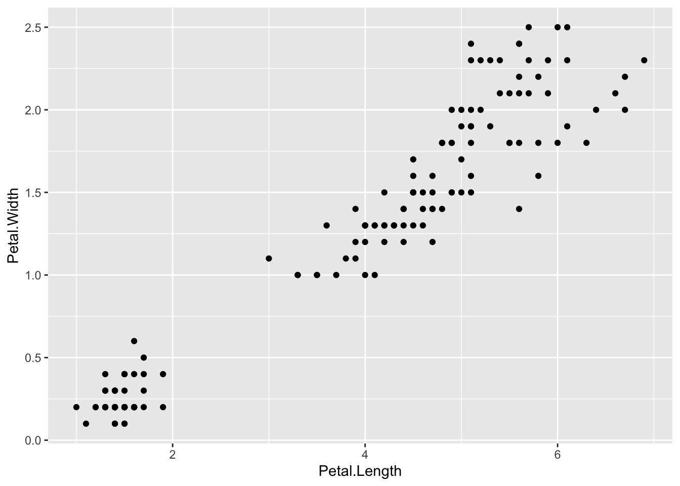
# -----------------------------# Load fonts (optional)# -----------------------------if ("extrafont"%in%installed.packages()[, "Package"]) {# Only try to load fonts if extrafont is installedsuppressMessages(loadfonts()) # suppress messages during Quarto render}# -----------------------------# Data loading and plots # -----------------------------data("iris")head(iris)
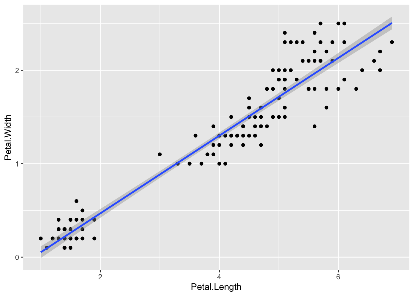
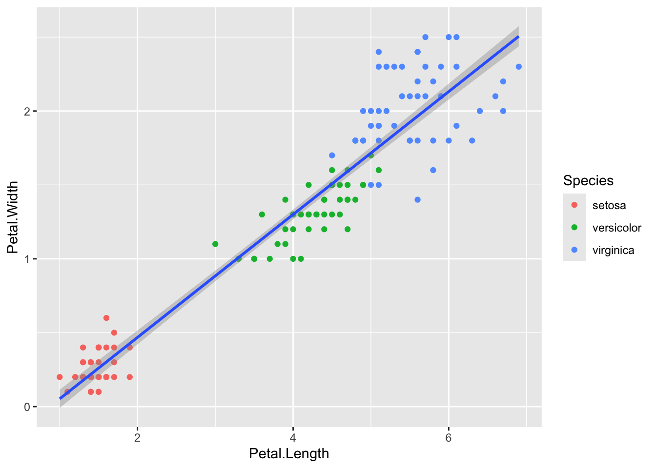
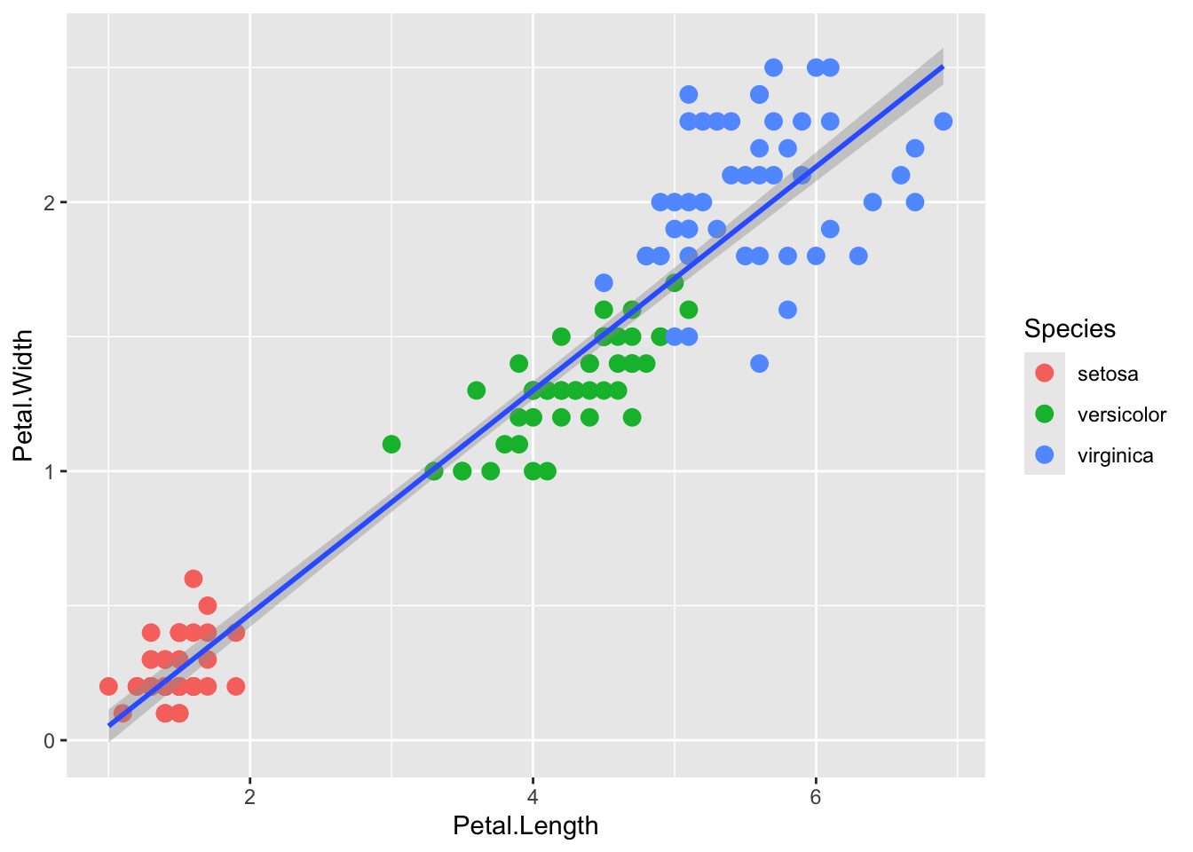
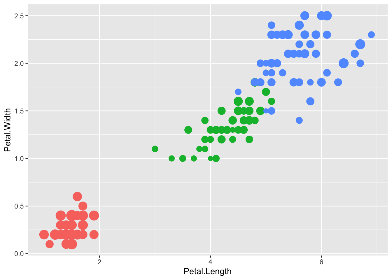
ggplot(data=iris,mapping=aes(x=Petal.Length,y=Petal.Width))+geom_point(aes(color=Species))+geom_smooth(method="lm") #add colours but keep only one regression line
`geom_smooth()` using formula = 'y ~ x'
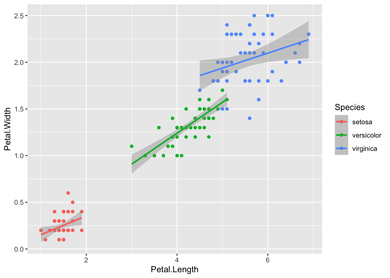
ggplot(data=iris,mapping=aes(x=Petal.Length,y=Petal.Width))+geom_point(aes(color=Species),size=3)+geom_smooth(method="lm") #change the size of the points
`geom_smooth()` using formula = 'y ~ x'
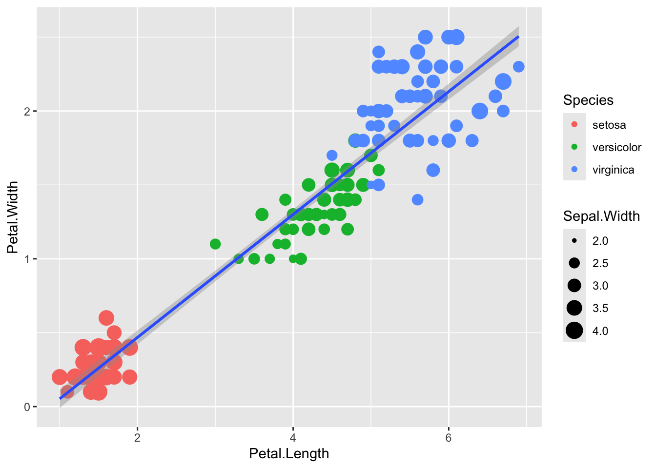
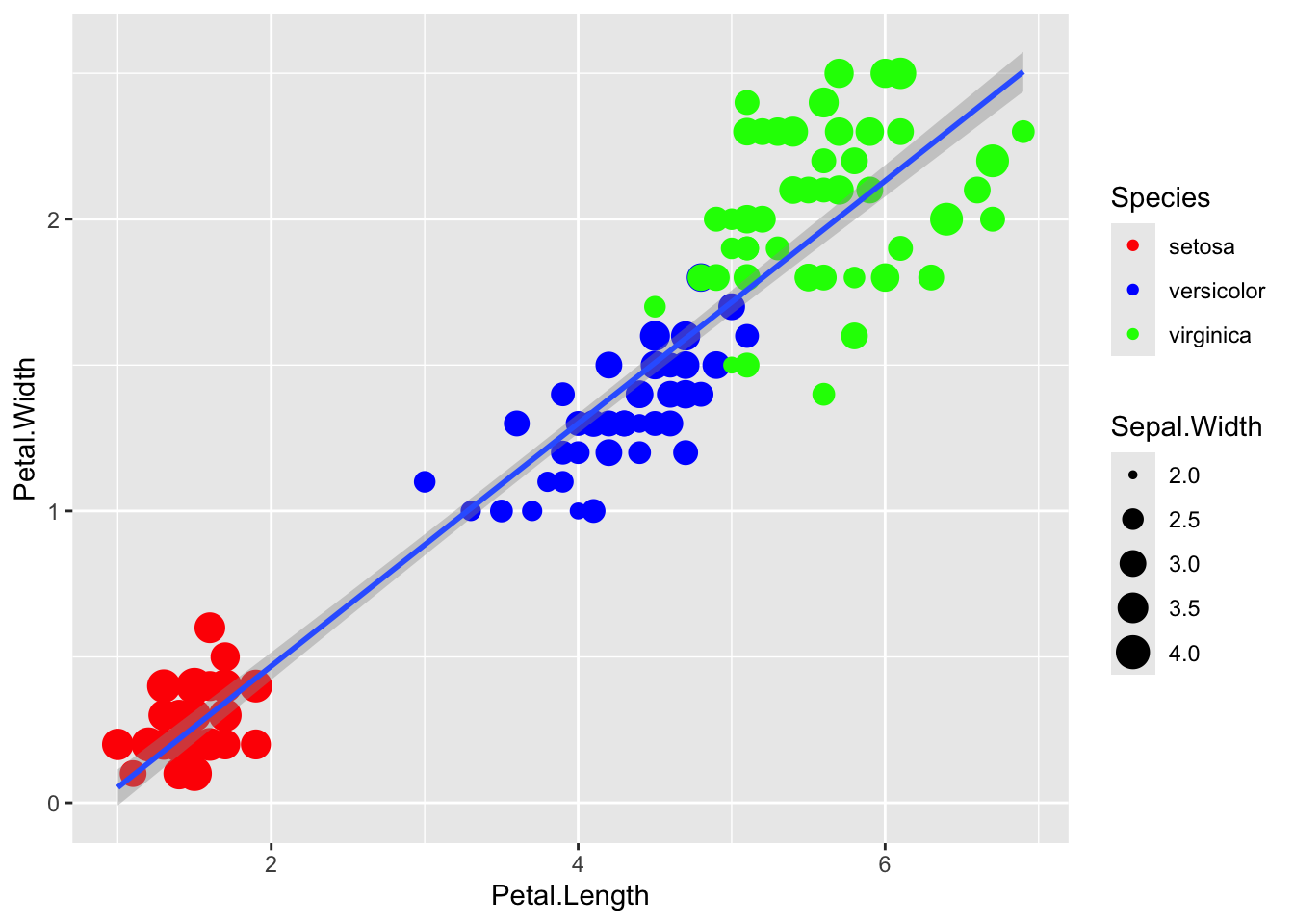
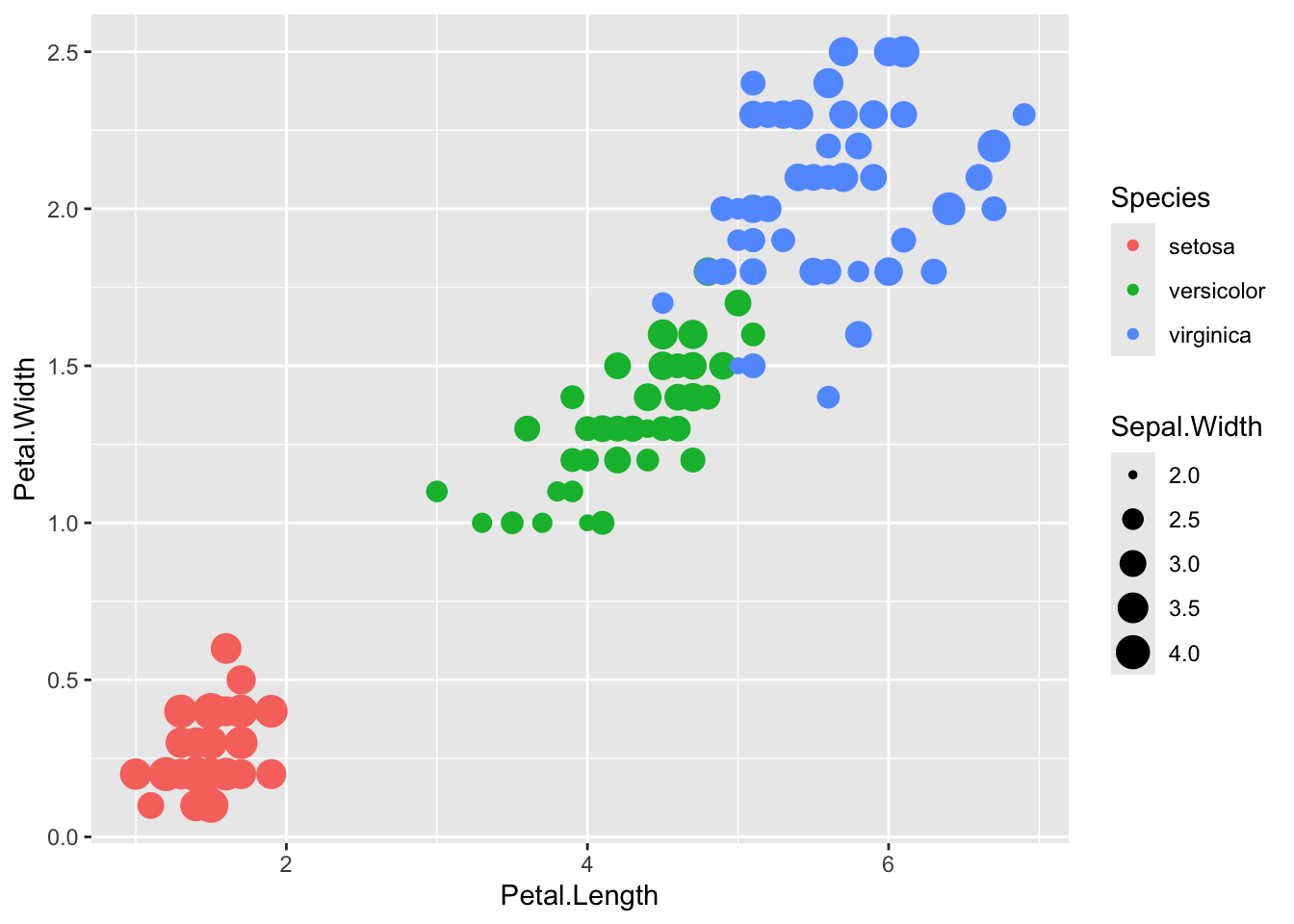
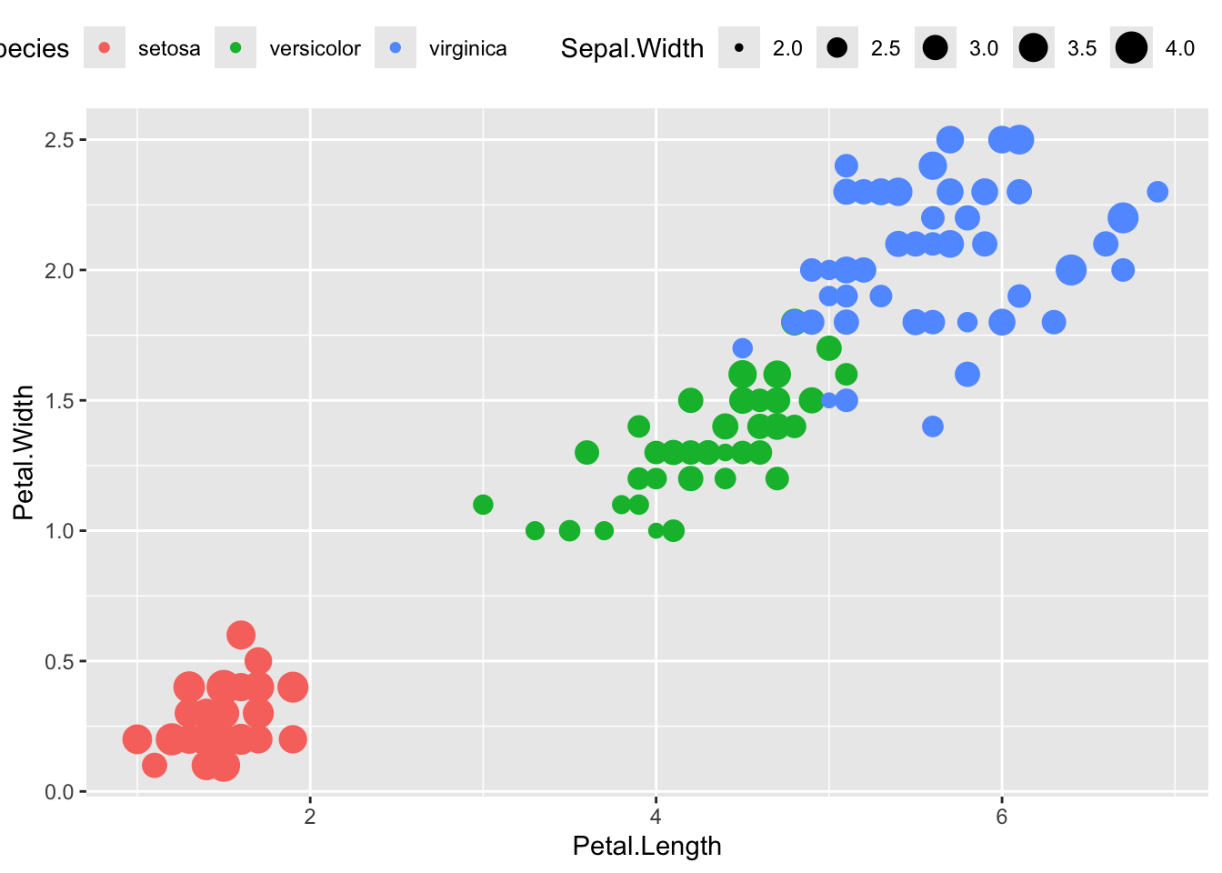
ggplot(data=iris,mapping=aes(x=Petal.Length,y=Petal.Width))+geom_point(aes(color=Species,size=Sepal.Width))+geom_smooth(method="lm") #add another subgoup, in this case the sepal.width
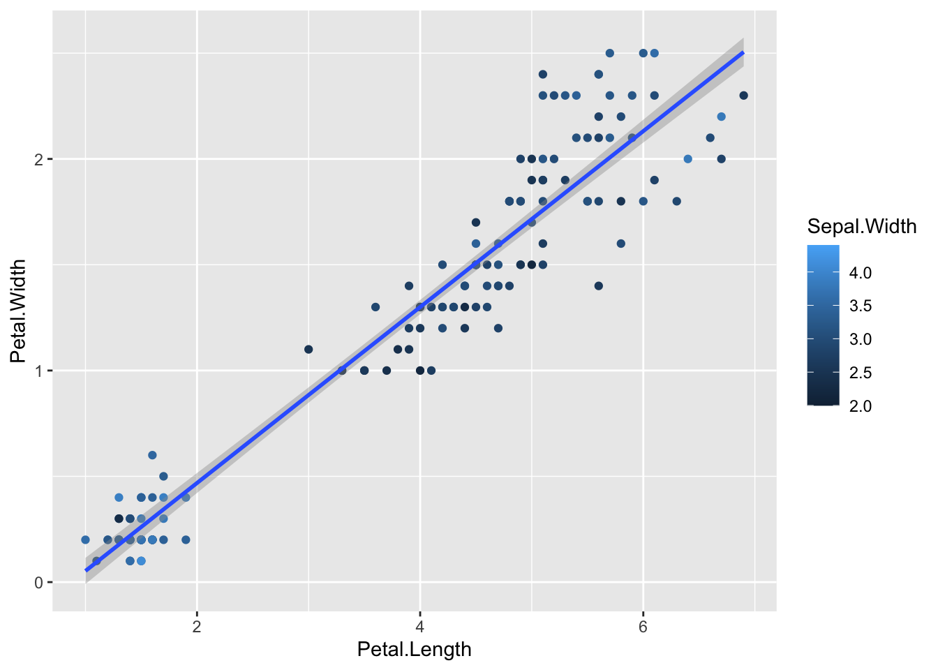
ggplot(data=iris,mapping=aes(x=Petal.Length,y=Petal.Width))+geom_point(aes(color=Sepal.Width))+geom_smooth(method="lm") #map the colours to a continous variable
`geom_smooth()` using formula = 'y ~ x'
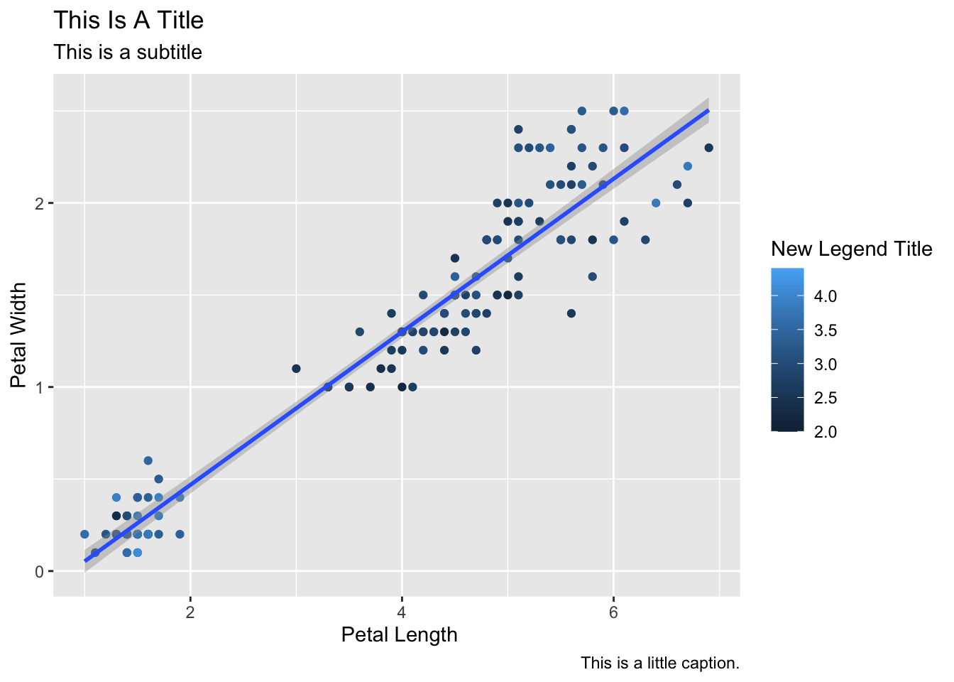
ggplot(data=iris,mapping=aes(x=Petal.Length,y=Petal.Width))+geom_point(aes(color=Sepal.Width))+geom_smooth(method="lm")+scale_color_continuous(name="New Legend Title")+labs(title="This Is A Title",subtitle="This is a subtitle",x=" Petal Length", y="Petal Width", caption="This is a little caption.") #add titles
`geom_smooth()` using formula = 'y ~ x'
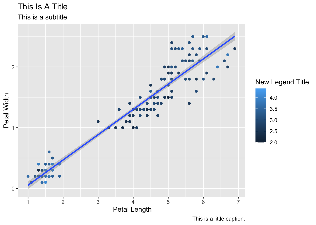
ggplot(data=iris,mapping=aes(x=Petal.Length,y=Petal.Width))+geom_point(aes(color=Sepal.Width))+geom_smooth(method="lm")+scale_color_continuous(name="New Legend Title")+scale_x_continuous(breaks=1:8)+labs(title="This Is A Title",subtitle="This is a subtitle",x=" Petal Length", y="Petal Width", caption="This is a little caption.") #modify the axis, start with 1,2,3
`geom_smooth()` using formula = 'y ~ x'
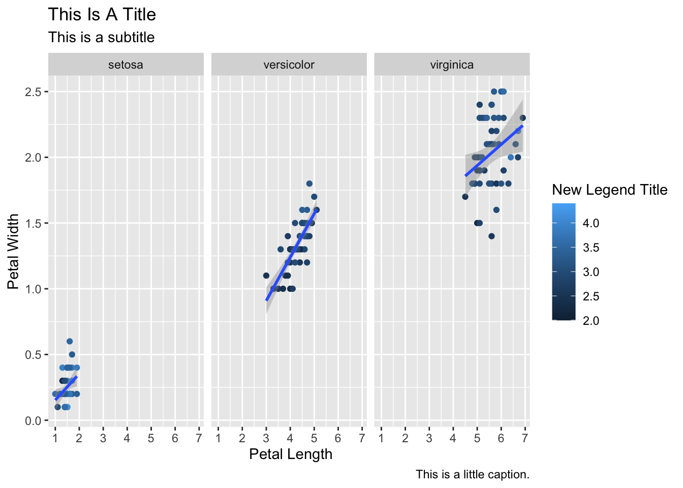
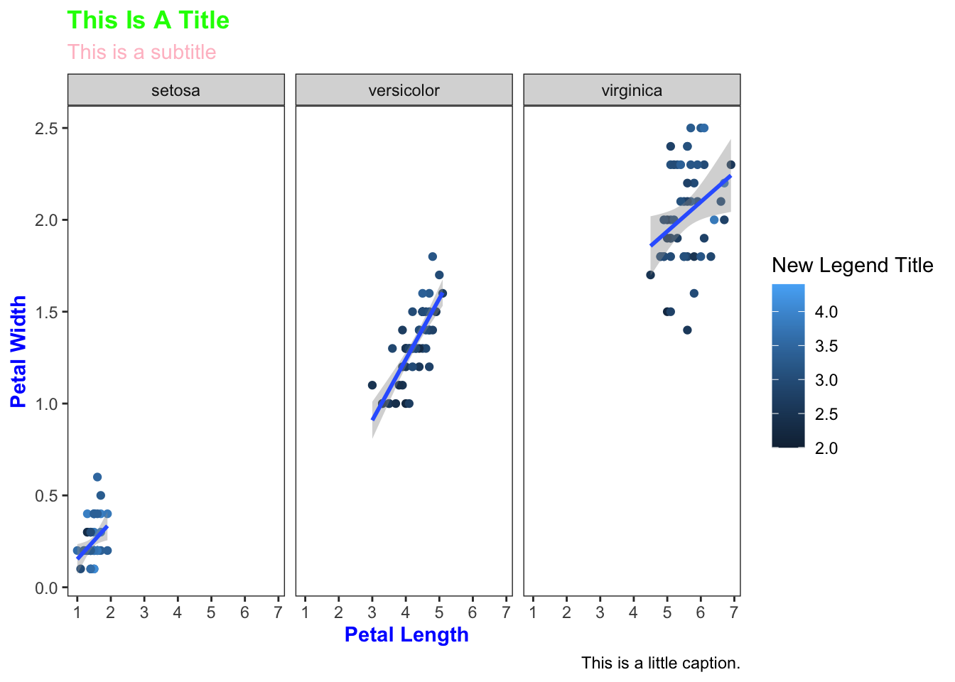
ggplot(data=iris,mapping=aes(x=Petal.Length,y=Petal.Width))+geom_point(aes(color=Sepal.Width))+geom_smooth(method="lm")+scale_color_continuous(name="New Legend Title")+scale_x_continuous(breaks=1:8)+labs(title="This Is A Title",subtitle="This is a subtitle",x=" Petal Length", y="Petal Width", caption="This is a little caption.")+facet_wrap(~Species) #create subplots using faceting function
`geom_smooth()` using formula = 'y ~ x'
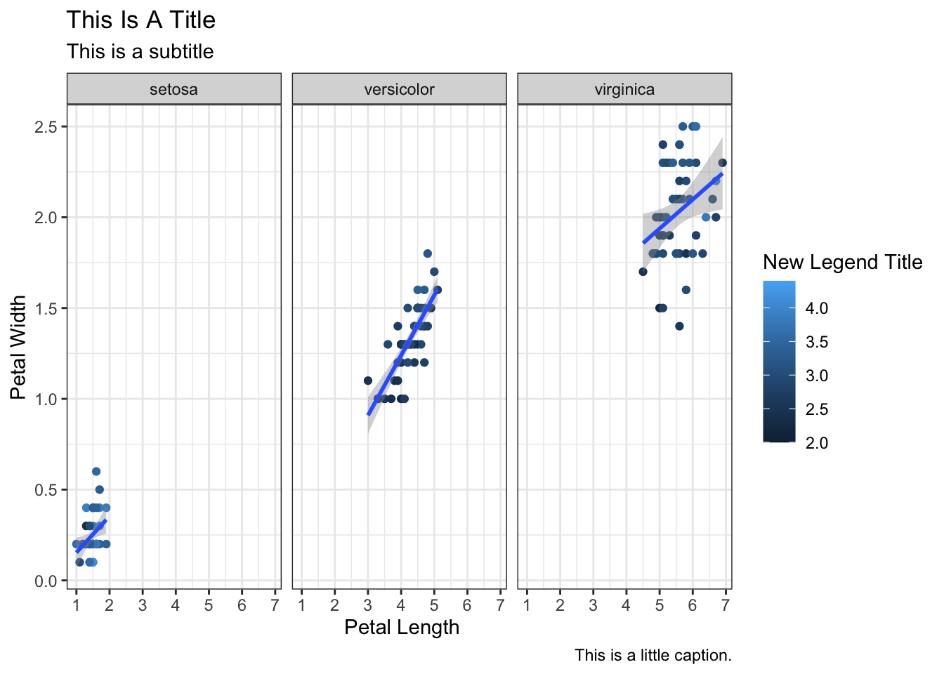
ggplot(data=iris,mapping=aes(x=Petal.Length,y=Petal.Width))+geom_point(aes(color=Sepal.Width))+geom_smooth(method="lm")+scale_color_continuous(name="New Legend Title")+scale_x_continuous(breaks=1:8)+labs(title="This Is A Title",subtitle="This is a subtitle",x=" Petal Length", y="Petal Width", caption="This is a little caption.")+facet_wrap(~Species)+theme_bw() #change the look of the plot by using the default theme_bw option
`geom_smooth()` using formula = 'y ~ x'
ggplot(data=iris,mapping=aes(x=Petal.Length,y=Petal.Width))+geom_point(aes(color=Sepal.Width))+geom_smooth(method="lm")+scale_color_continuous(name="New Legend Title")+scale_x_continuous(breaks=1:8)+labs(title="This Is A Title",subtitle="This is a subtitle",x=" Petal Length", y="Petal Width", caption="This is a little caption.")+facet_wrap(~Species)+theme_bw()+theme(axis.title=element_text(color="Blue",face="bold"),plot.title=element_text(color="Green",face="bold"),plot.subtitle=element_text(color="Pink"),panel.grid=element_blank() ) #use the theme to chnage the colours of the axis and title/subtitle
`geom_smooth()` using formula = 'y ~ x'
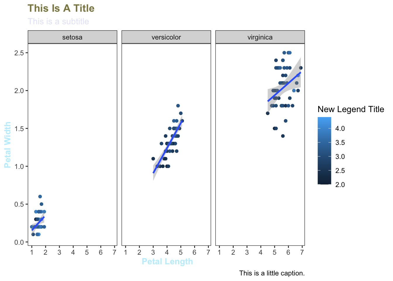
newtheme <-theme(axis.title=element_text(color="lightblue1",face="bold"),plot.title=element_text(color="khaki4",face="bold"),plot.subtitle=element_text(color="lavender"),panel.grid=element_blank()) #this will save the theme and afterwards this same theme can be reusedggplot(data=iris,mapping=aes(x=Petal.Length,y=Petal.Width))+geom_point(aes(color=Sepal.Width))+geom_smooth(method="lm")+scale_color_continuous(name="New Legend Title")+scale_x_continuous(breaks=1:8)+labs(title="This Is A Title",subtitle="This is a subtitle",x=" Petal Length", y="Petal Width", caption="This is a little caption.")+facet_wrap(~Species)+theme_bw()+ newtheme
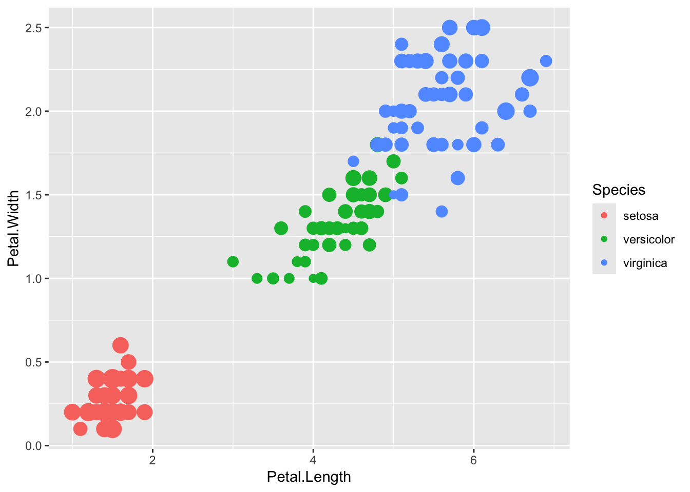
ggplot(data=iris,mapping=aes(x=Petal.Length,y=Petal.Width))+geom_point(aes(color=Species,size=Sepal.Width))+guides(size="none") #we removed one legend
ggplot(data=iris,mapping=aes(x=Petal.Length,y=Petal.Width))+geom_point(aes(color=Species,size=Sepal.Width),show.legend=FALSE) #turning off both legends using geom
ggplot(data=iris,mapping=aes(x=Petal.Length,y=Petal.Width))+geom_point(aes(color=Species,size=Sepal.Width))+theme(legend.position="top",legend.justification="right") #use theme to move the position of the legends
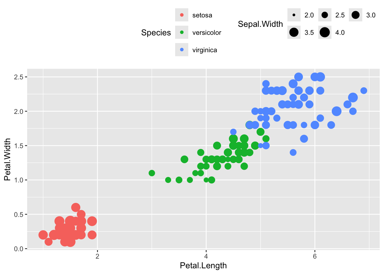
ggplot(data=iris,mapping=aes(x=Petal.Length,y=Petal.Width))+geom_point(aes(color=Species,size=Sepal.Width))+guides(size=guide_legend(nrow=2,byrow=TRUE),color=guide_legend(nrow=3,byrow=T))+theme(legend.position="top",legend.justification="right") #control of the legends rows
ggplot(data=iris,mapping=aes(x=Petal.Length,y=Petal.Width))+geom_point(aes(color=Species))+geom_text(aes(label=Species,hjust=0),nudge_x=0.5,size=3) # add labels to the data/points
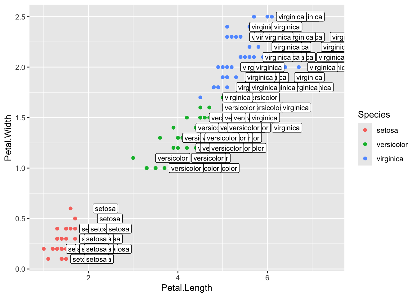
ggplot(data=iris,mapping=aes(x=Petal.Length,y=Petal.Width))+geom_point(aes(color=Species))+geom_label(aes(label=Species,hjust=0),nudge_x=0.5,size=3) #edit the labels theme
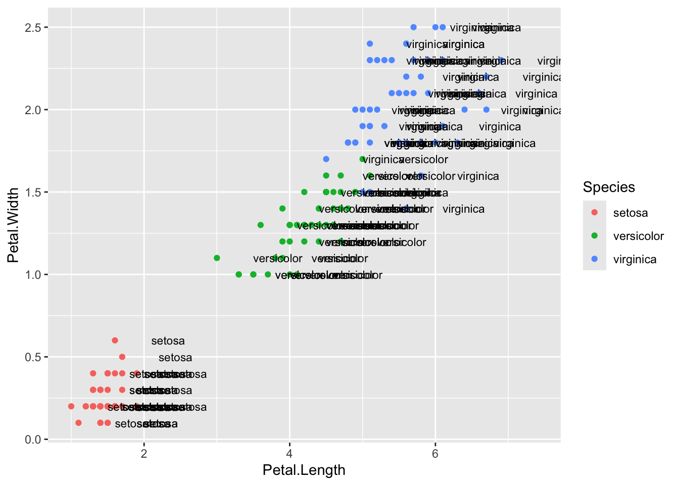
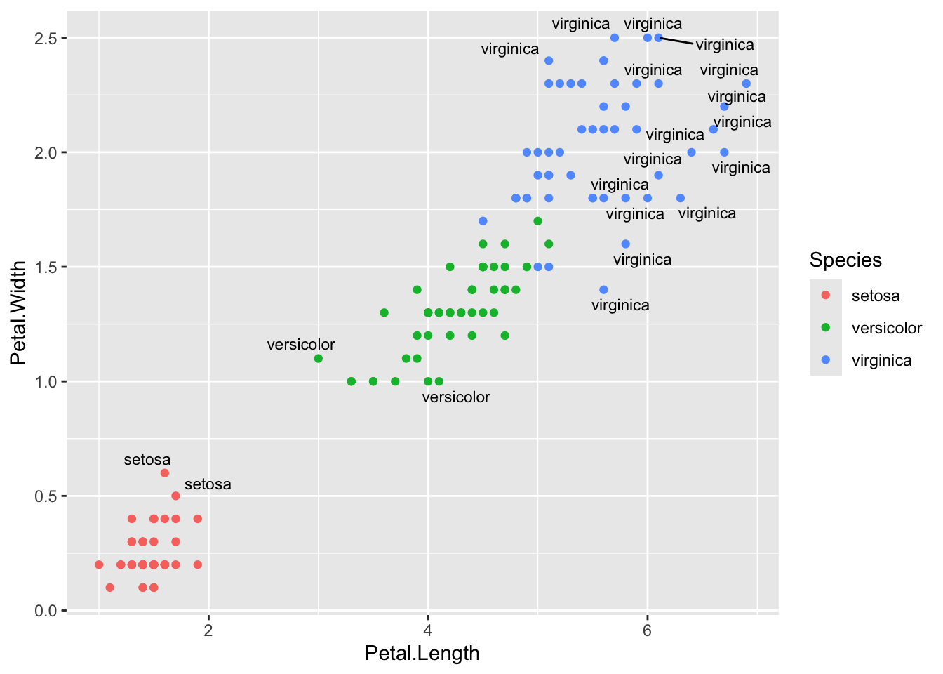
ggplot(data=iris,mapping=aes(x=Petal.Length,y=Petal.Width))+geom_point(aes(color=Species))+geom_text_repel(aes(label=Species),size=3) #use ggrepel to avoid having the labels overlapping
Warning: ggrepel: 130 unlabeled data points (too many overlaps). Consider
increasing max.overlaps
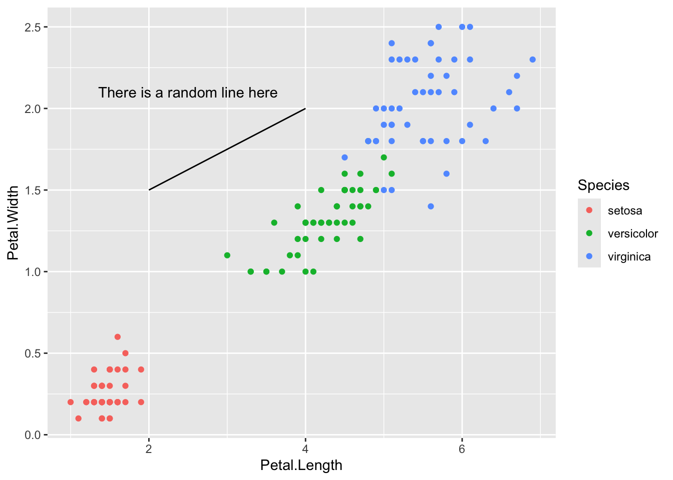
ggplot(data=iris,mapping=aes(x=Petal.Length,y=Petal.Width))+geom_point(aes(color=Species))+annotate("text",x=2.5,y=2.1,label="There is a random line here")+annotate("segment",x=2,xend=4,y=1.5,yend=2) #add customn annotations
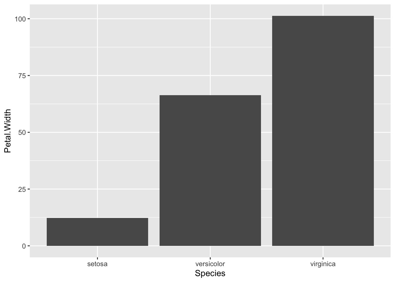
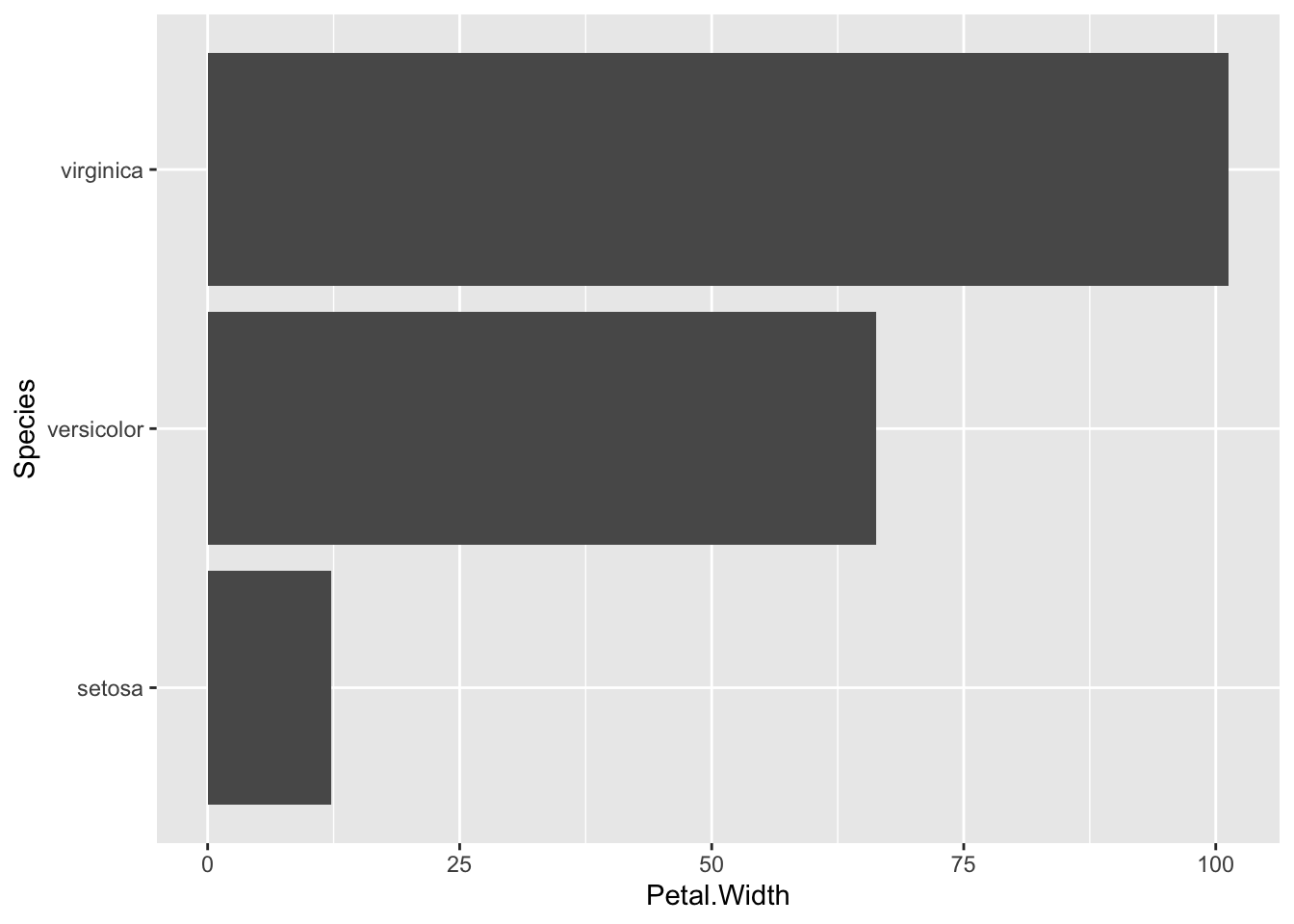
ggplot(data=iris,mapping=aes(x=Species,y=Petal.Width))+geom_bar(stat="identity")+coord_flip() #flip the axes
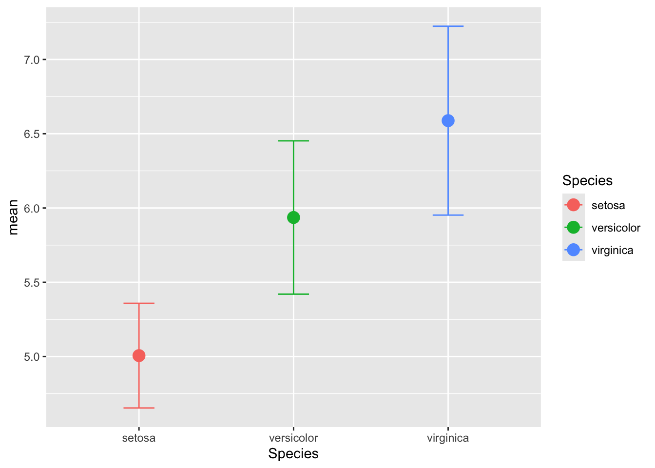
dfr <- iris %>%group_by(Species) %>%summarise(mean=mean(Sepal.Length),sd=sd(Sepal.Length)) %>%mutate(high=mean+sd,low=mean-sd) #mean and standard deviation ggplot(data=dfr,mapping=aes(x=Species,y=mean,color=Species))+geom_point(size=4)+geom_errorbar(aes(ymax=high,ymin=low),width=0.2) #plotting the error bars
###### ECONOMIST SCATTERPLOT #######ec <-read.csv("/Users/lara/Downloads/data_economist.csv",header=T) #import the data from the .csv filehead(ec) #read the data
  X     Country HDI.Rank   HDI CPI            Region
1 1 Afghanistan      172 0.398 1.5      Asia Pacific
2 2     Albania       70 0.739 3.1 East EU Cemt Asia
3 3     Algeria       96 0.698 2.9              MENA
4 4      Angola      148 0.486 2.0               SSA
5 5   Argentina       45 0.797 3.0          Americas
6 6     Armenia       86 0.716 2.6 East EU Cemt Asia
str(ec) #check that HDI and CPI are numerical variables and Region is a categorical one/factor
'data.frame':   173 obs. of  6 variables:
 $ X       : int  1 2 3 4 5 6 7 8 9 10 ...
 $ Country : chr  "Afghanistan" "Albania" "Algeria" "Angola" ...
 $ HDI.Rank: int  172 70 96 148 45 86 2 19 91 53 ...
 $ HDI     : num  0.398 0.739 0.698 0.486 0.797 0.716 0.929 0.885 0.7 0.771 ...
 $ CPI     : num  1.5 3.1 2.9 2 3 2.6 8.8 7.8 2.4 7.3 ...
 $ Region  : chr  "Asia Pacific" "East EU Cemt Asia" "MENA" "SSA" ...
levels(ec$Region) # we can't see the levels, therefore we need to modify the Regions variable
NULL
ec$Region <-factor(ec$Region,levels =c("EU W. Europe","Americas","Asia Pacific","East EU Cemt Asia","MENA","SSA"),labels =c("OECD","Americas","Asia &\nOceania","Central &\nEastern Europe","Middle East &\nNorth Africa","Sub-Saharan\nAfrica")) #use factor levels and labels to rename factorslevels(ec$Region) #check that we have made the change
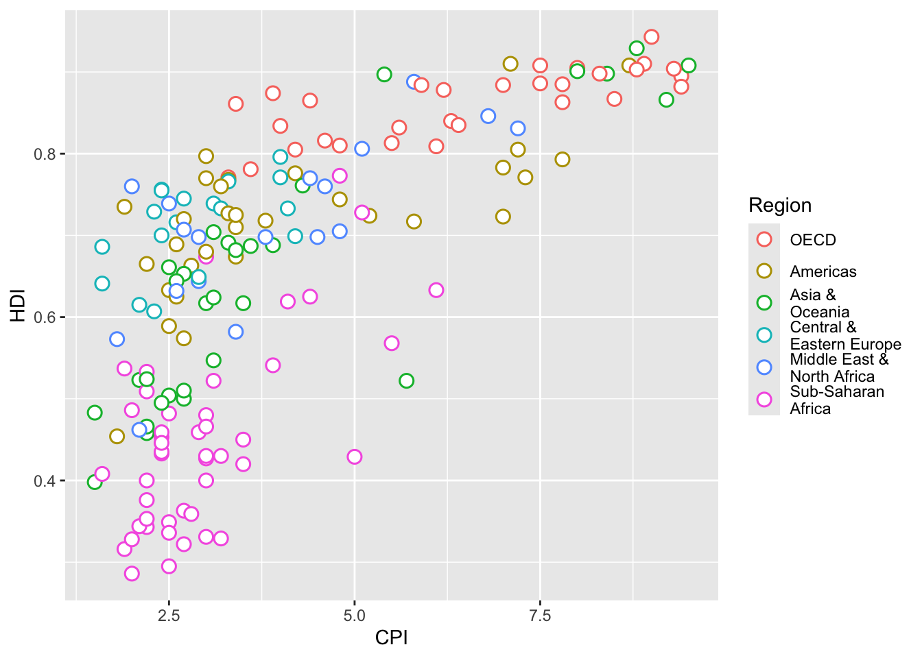
ggplot(ec,aes(x=CPI,y=HDI,color=Region))+geom_point(shape=21,size=3,stroke=0.8,fill="white") #generate a plot with points without fill.
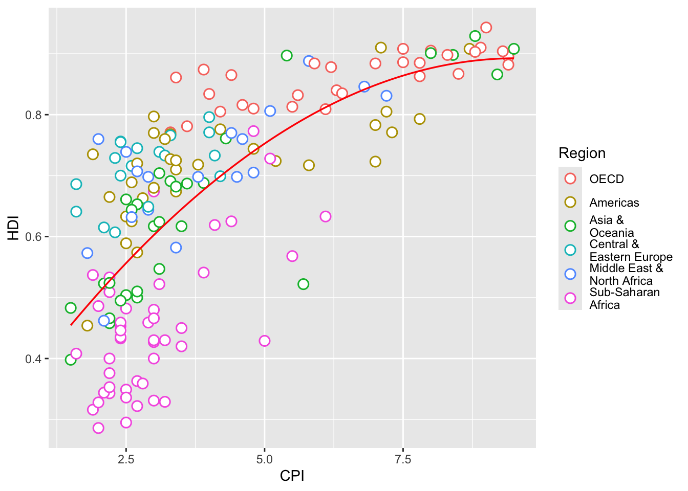
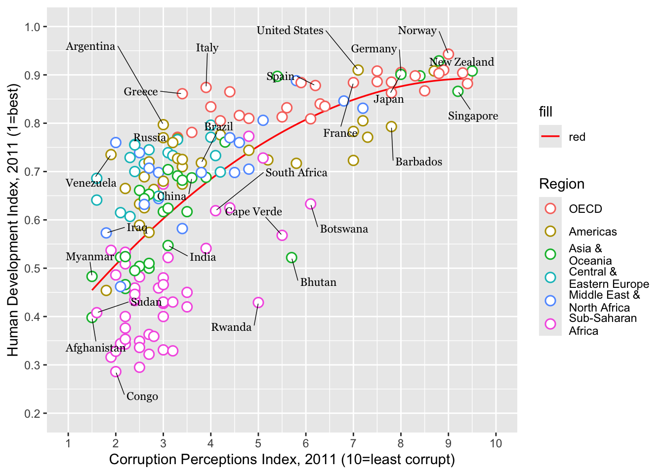
ggplot(ec,aes(x=CPI,y=HDI,color=Region))+geom_point(shape=21,size=3,stroke=0.8,fill="white")+geom_smooth(method="lm",formula=y~poly(x,2),se=F,size=0.6,color="red") #add a trendline in red
Warning: Using `size` aesthetic for lines was deprecated in ggplot2 3.4.0.
ℹ Please use `linewidth` instead.
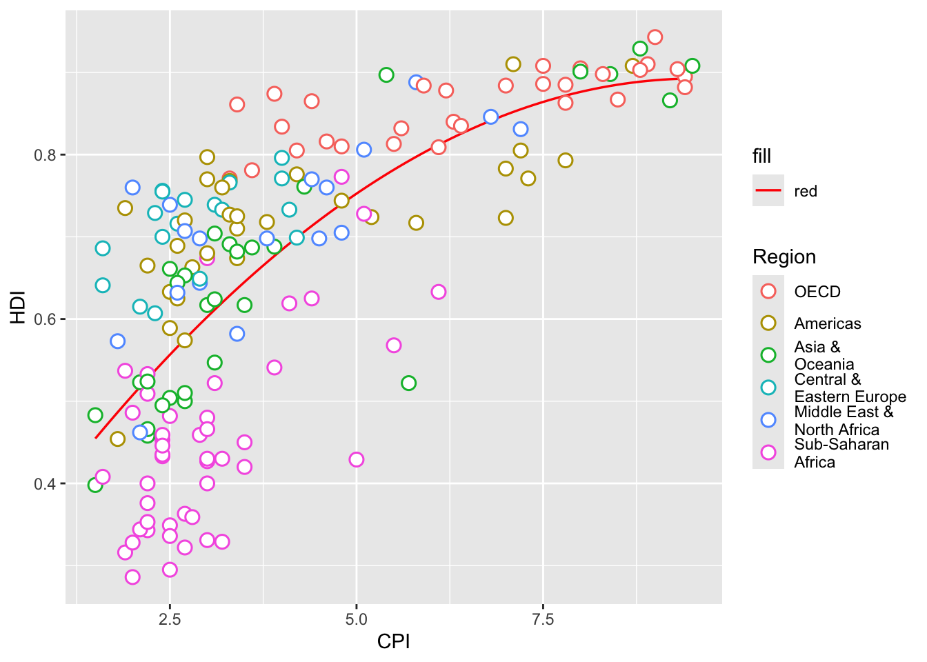
p <-ggplot(ec,aes(x=CPI,y=HDI,color=Region))+geom_smooth(aes(fill="red"),method="lm",formula=y~poly(x,2),se=F,color="red",size=0.6)+geom_point(shape=21,size=3,stroke=0.8,fill="white") #we want the points on top of the line so we assign the plot to a variable and alter the order of geom_smooth and geom_pointp #to print/see the plot
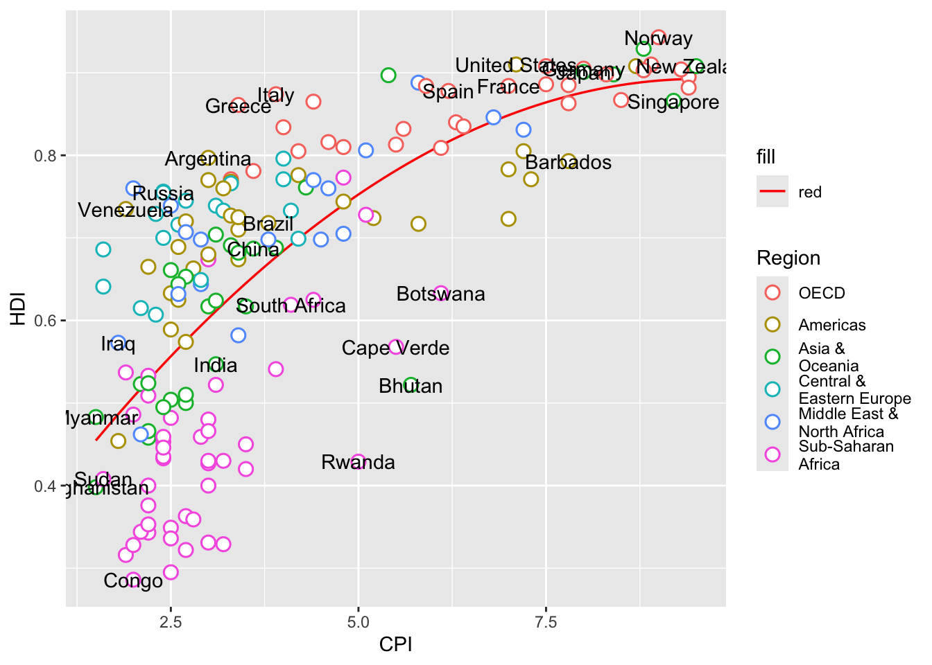
labels <-c("Congo","Afghanistan","Sudan","Myanmar","Iraq","Venezuela","Russia","Argentina","Brazil","Italy","South Africa","Cape Verde","Bhutan","Botswana","Britian","New Zealand","Greece","China","India","Rwanda","Spain","France","United States","Japan","Norway","Singapore","Barbados","Germany")p+geom_text(data=subset(ec,Country %in% labels),aes(label=Country),color="black") #add the labels to the new coutries on the plot
#########IF YOU WAN TO CHANGE THE FONT font_import(pattern="Georgia",prompt=FALSE)
Scanning ttf files in /Library/Fonts/, /System/Library/Fonts, /System/Library/Fonts/Supplemental, ~/Library/Fonts/ ...
Extracting .afm files from .ttf files...
/System/Library/Fonts/SFGeorgian.ttf : -SFGeorgian-Regular already registered in fonts database. Skipping.
/System/Library/Fonts/SFGeorgianRounded.ttf : -SFGeorgianRounded-Regular already registered in fonts database. Skipping.
/System/Library/Fonts/Supplemental/Georgia Bold Italic.ttf : Georgia-BoldItalic already registered in fonts database. Skipping.
/System/Library/Fonts/Supplemental/Georgia Bold Italic.ttf : Georgia-BoldItalic already registered in fonts database. Skipping.
/System/Library/Fonts/Supplemental/Georgia Bold.ttf : Georgia-Bold already registered in fonts database. Skipping.
/System/Library/Fonts/Supplemental/Georgia Bold.ttf : Georgia-Bold already registered in fonts database. Skipping.
/System/Library/Fonts/Supplemental/Georgia Italic.ttf : Georgia-Italic already registered in fonts database. Skipping.
/System/Library/Fonts/Supplemental/Georgia Italic.ttf : Georgia-Italic already registered in fonts database. Skipping.
/System/Library/Fonts/Supplemental/Georgia.ttf : Georgia already registered in fonts database. Skipping.
/System/Library/Fonts/Supplemental/Georgia.ttf : Georgia already registered in fonts database. Skipping.
Found FontName for 0 fonts.
Scanning afm files in /Library/Frameworks/R.framework/Versions/4.5-arm64/Resources/library/extrafontdb/metrics
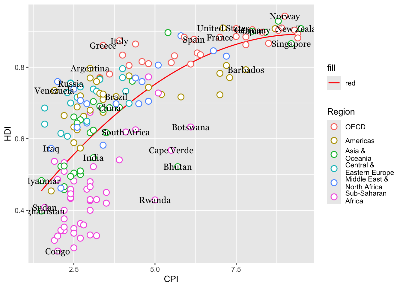
# load fonts for pdf#loadfonts()# list available fonts in R#fonts()########p+geom_text(data=subset(ec,Country %in% labels),aes(label=Country),color="black",family="Georgia") #change the font of the labels
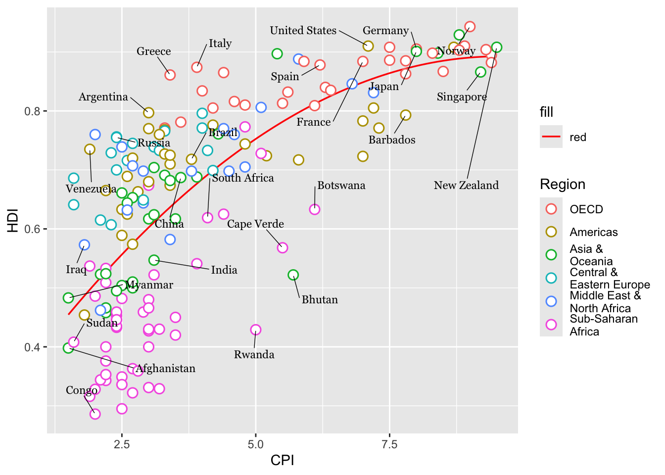
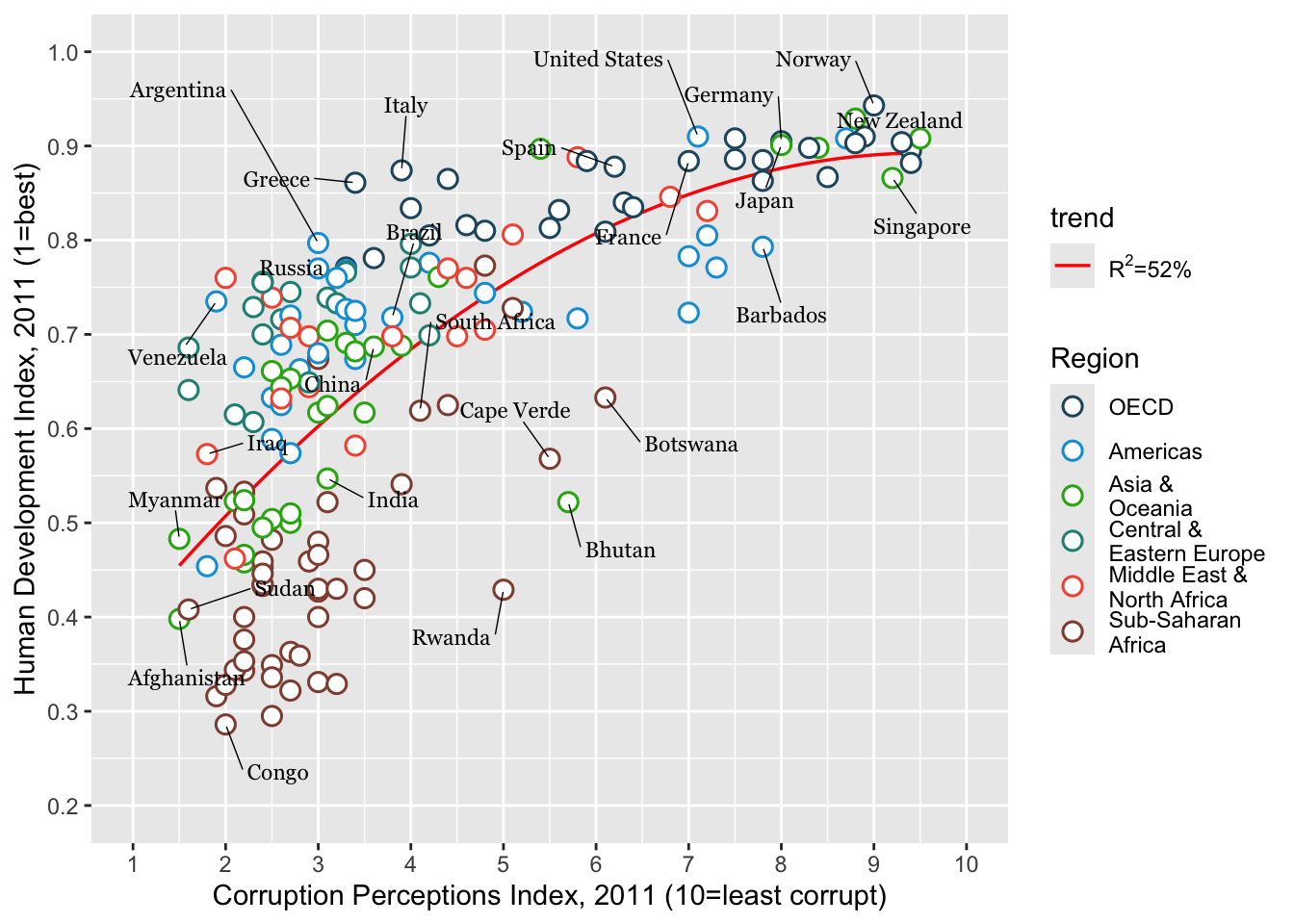
library(ggrepel)p <- p+geom_text_repel(data=subset(ec,Country %in% labels),aes(label=Country),color="black",box.padding=unit(1,'lines'),segment.size=0.25,size=3,family="Georgia") #solve the overlap of the labelsp
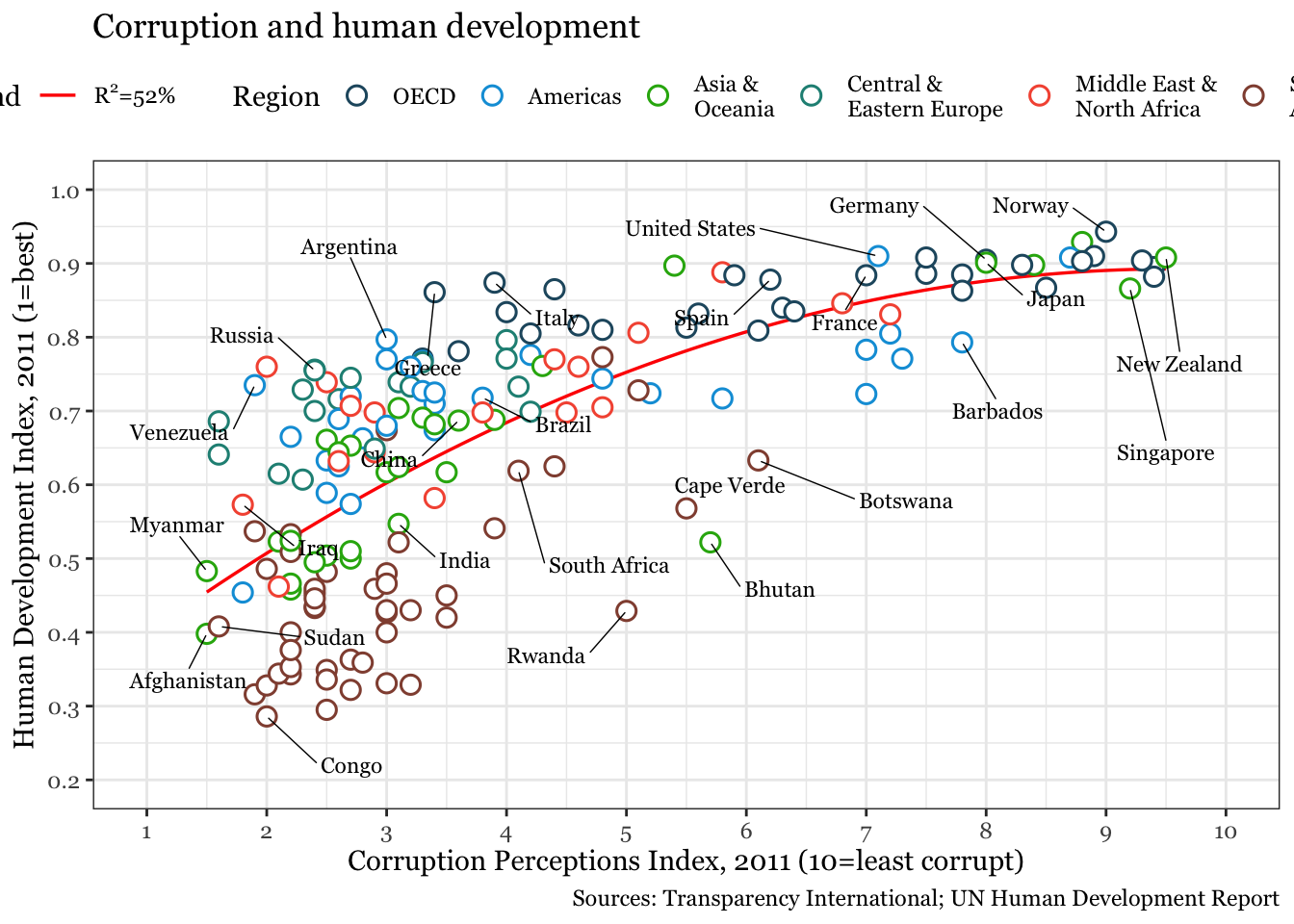
p <- p+scale_x_continuous(name="Corruption Perceptions Index, 2011 (10=least corrupt)",breaks=1:10,limits=c(1,10))+scale_y_continuous(name="Human Development Index, 2011 (1=best)",breaks=seq(from=0,to=1,by=0.1),limits=c(0.2,1)) #adjust the axesp
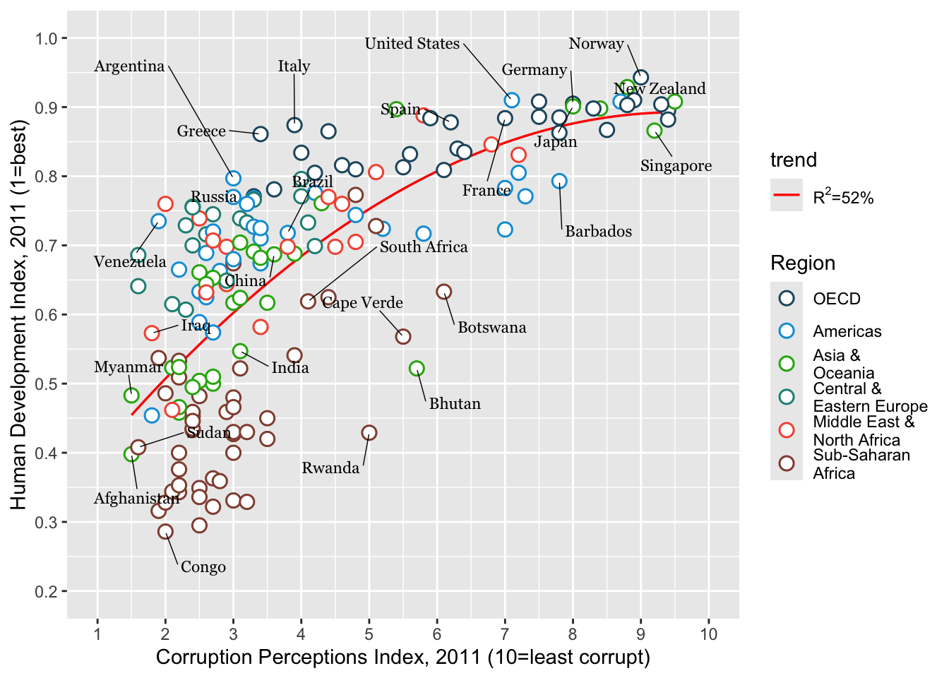
p <- p+scale_color_manual(values=c("#23576E","#099FDB","#29B00E", "#208F84","#F55840","#924F3E"))+scale_fill_manual(name="trend",values="red",labels=expression(paste(R^2,"=52%"))) #to change the colors of the points and the red fill label p
#I don't want to change the colors so I'm just going to add the new labelp <- p+scale_fill_manual(name="trend",values="red",labels=expression(paste(R^2,"=52%")))
Scale for fill is already present.
Adding another scale for fill, which will replace the existing scale.
p
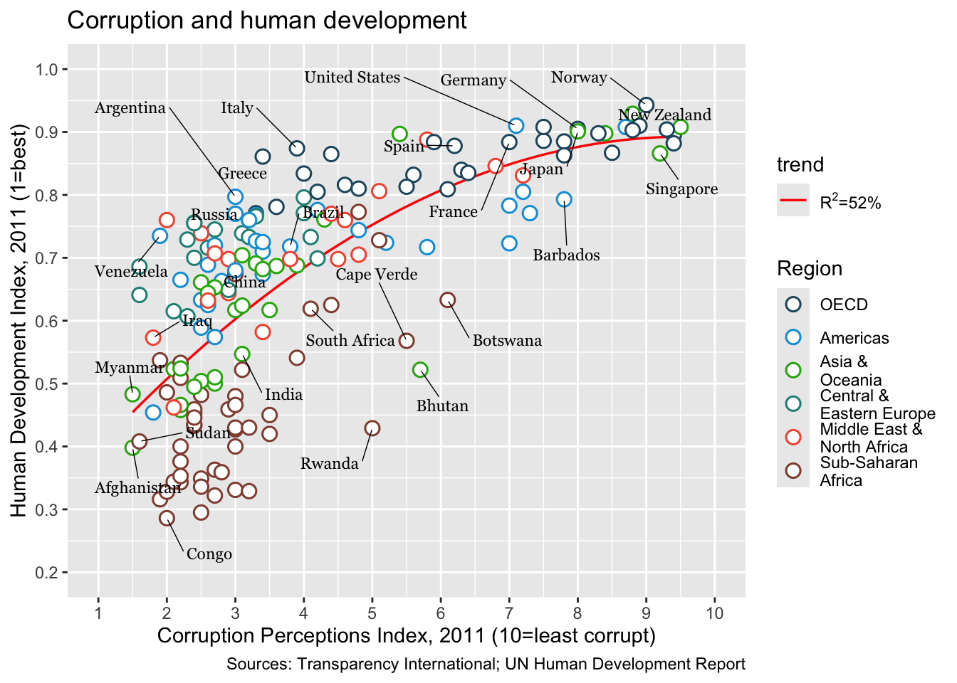
p <- p+labs(title="Corruption and human development",caption="Sources: Transparency International; UN Human Development Report") #add a title to the plot p
p <- p+guides(color=guide_legend(nrow=1))+theme_bw(base_family="Georgia")+theme(legend.position="top") #move the legend to the top and change the font in all the textp
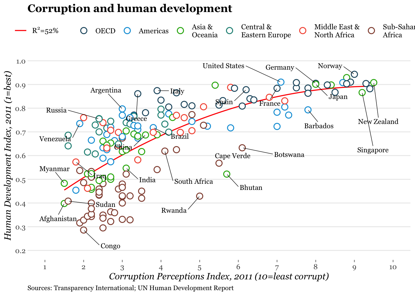
### Now we do some careful refining with themes.#Turn off minor gridlines#Turn off major gridlines on x-axis#Remove the gray background#Remove panel border#Remove legend titles#Make axes titles italic#Turn off y-axis ticks#Change x-axis ticks to color grey60#Make plot title bold#Decrease size of caption to size 8p+theme(panel.grid.minor=element_blank(),panel.grid.major.x=element_blank(),panel.background=element_blank(),panel.border=element_blank(),legend.title=element_blank(),axis.title=element_text(face="italic"),axis.ticks.y=element_blank(),axis.ticks.x=element_line(color="grey60"),plot.title=element_text(face="bold"),plot.caption=element_text(hjust=0,size=8))